Deutsch-Jozsa Algorithm

Deutsch-Jozsa algorithm (Qualitative)

Deutsch’s algorithm is one of the simplest examples showing how quantum computers can outperform classical computers — even on a very small problem.

It deals with a special kind of function:

\[ f(x): \{0,1\}^n \rightarrow \{0,1\} \]

and tries to determine whether \( f(x) \) is:

Constant: the output is always the same (either always 0 or always 1), or
Balanced: the output is 0 for half of the possible inputs and 1 for the other half.

In classical computing, you would need to check more than one input to be sure which type of function it is. But Deutsch–Jozsa algorithm takes advantage of quantum parallelism — it evaluates the function for all possible inputs at once, using the principle of superposition.

Then, using quantum interference, it determines whether the function is constant or balanced with just one evaluation. This makes it one of the first and clearest demonstrations of quantum speed-up — solving a problem in a single quantum step that would take multiple classical steps.

Deutsch-Jozsa algorithm (Quantitative)

Deutsch's algorithm is one of the simplest quantum algorithms, demonstrating the power of quantum parallelism and interference. It solves a specific problem—determining whether a function 𝑓(𝑥) is constant or balanced—more efficiently than any classical algorithm.

Given a function 𝑓(𝑥) where:

𝑓(𝑥):{0,1}ⁿ→{0,1}

determine whether 𝑓(𝑥) is:

Constant: f(x) has the same output (either 0 or 1) for all 𝑥, or
Balanced: f(x) outputs 0 for half the inputs and 1 for the other half.

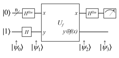
Quantum Circuit for Deutsch-Jozsa Algorithm

1. Initialize Qubits:

\( |\psi_0\rangle = |00\cdots0\rangle \otimes |1\rangle \)

\( |\psi_0\rangle = |0\rangle^{\otimes n} |1\rangle \)

2. Apply Hadamard Gates:

\( |\psi_1\rangle = H^{\otimes n} |0\rangle^{\otimes n} \, H|1\rangle \)

\( |\psi_1\rangle = H|00\cdots0\rangle \otimes H|1\rangle \)

\( |\psi_1\rangle = \frac{1}{\sqrt{2}} (|0\rangle + |1\rangle) \otimes \frac{1}{\sqrt{2}} (|0\rangle + |1\rangle) \otimes \cdots \otimes \frac{1}{\sqrt{2}} (|0\rangle + |1\rangle) |-\rangle \)

For Two Qubits

\( H^{\otimes 2} |0\rangle^{\otimes 2} = \frac{1}{\sqrt{2}} (|0\rangle + |1\rangle) \otimes \frac{1}{\sqrt{2}} (|0\rangle + |1\rangle) \)

\( H^{\otimes 2} |0\rangle^{\otimes 2} = \frac{1}{\sqrt{2^2}} ( |00\rangle + |01\rangle + |10\rangle + |11\rangle ) \)

\( H^{\otimes 2} |0\rangle^{\otimes 2} = \frac{1}{\sqrt{2^2}} \sum_{x \in \{0,1\}^2} |x\rangle \)

For Three Qubits

\( H^{\otimes 3} |0\rangle^{\otimes 3} = \frac{1}{\sqrt{2^3}} ( |000\rangle + |001\rangle + |010\rangle + |011\rangle + |100\rangle + |101\rangle + |110\rangle + |111\rangle ) \)

\( H^{\otimes 3} |0\rangle^{\otimes 3} = \frac{1}{\sqrt{2^3}} \sum_{x \in \{0,1\}^3} |x\rangle \)

3. Apply Oracle \( U_f \)

\( |\psi_2\rangle = U_f \frac{1}{\sqrt{2^n}} \sum_{x \in \{0,1\}^n} |x\rangle |-\rangle \)

\( |\psi_2\rangle = \frac{1}{\sqrt{2^n}} \sum_{x \in \{0,1\}^n} U_f |x\rangle |-\rangle \qquad U_f |x\rangle |-\rangle = (-1)^{f(x)} |x\rangle |-\rangle \)

\( |\psi_2\rangle = \frac{1}{\sqrt{2^n}} \sum_{x \in \{0,1\}^n} (-1)^{f(x)} |x\rangle |-\rangle \)

4. Apply Hadamard Gate

\( |\psi_3\rangle = \frac{1}{\sqrt{2^n}} \sum_{x \in \{0,1\}^n} (-1)^{f(x)} H^{\otimes n} |x\rangle |-\rangle \)

\( H^{\otimes n} |x\rangle = H|x_0\rangle \otimes H|x_1\rangle \otimes \cdots \otimes H|x_{n-1}\rangle \)

\( H |x_i\rangle = \frac{1}{\sqrt{2}} ( |0\rangle + (-1)^{x_i} |1\rangle ) \)

\( H|0\rangle = \frac{1}{\sqrt{2}} ( |0\rangle + |1\rangle ) \)

\( H|1\rangle = \frac{1}{\sqrt{2}} ( |0\rangle - |1\rangle ) \)

Testing \( H^{\otimes 3} |x\rangle \)

\( H^{\otimes 3} |x\rangle = H|x_0\rangle \otimes H|x_1\rangle \otimes H|x_2\rangle \)

\( = \frac{1}{\sqrt{2}} (|0\rangle + (-1)^{x_0}|1\rangle) \otimes \frac{1}{\sqrt{2}} (|0\rangle + (-1)^{x_1}|1\rangle) \otimes \frac{1}{\sqrt{2}} (|0\rangle + (-1)^{x_2}|1\rangle) \)

\( = \frac{1}{\sqrt{2^3}} \sum_{z \in \{0,1\}^3} (-1)^{x \cdot z} |z\rangle \)

where the dot product is \( x \cdot z = x_0 z_0 + x_1 z_1 + x_2 z_2 \).

Generalization

\( H^{\otimes n} |x\rangle = \frac{1}{\sqrt{2^n}} \sum_{z \in \{0,1\}^n} (-1)^{x \cdot z} |z\rangle \)

Effect on \( |\psi_3\rangle \)